An Introduction to Machine Learning Interpretability
Lately there has been a lot of interest in explainable AI/ML. Nobody wants to feel discriminated against by an algorithm and when we don't like its prediction or decision we want to know why it made that decision. Plus there is an added sense of security when we feel we understand (or could understand) how something works.
The concept of how well a human can understand the prediction of a machine learning model is often called interpretability or explainability. The two terms are often used interchangeably though I'm starting to strongly believe that interpretability is the better word for what we can do today.
There are several related but different concept here so let me point out that interpretability is related to Fairness which concerns a model being (socially) unbiased and not discriminating.
... It is related to Safety and Reliability which attempts to ensure that errors are not catastrophic and are expected and properly handled.
... It is related to Privacy which is concerned with protecting sensitive information.
... It is related to Justification which examines why a decision is a good decision.
... And it is related to and often used interchangeably with Explainabilty. However, I posit that explainability more closely means why something happened while interpretability tells us more about how things are correlated.
That is, when something goes wrong or we make an unexpected prediction your boss/client/user wants to know WHY and they want the explanation to be:
- monotonic - larger houses cost more vs you have too much experience
- homoscedastic - predictions are stable and accurate for all possible conditions
- not probabilistic - (I love probability distributions but) most people want a single number to focus on
- contrastive - why is that person get a loan but I didn't
- selective - what are the 3 most important reasons (not 100's of factors)
- perscriptive - what can I do to get a better score
- conformant to social expectations - explain it like I'm five
Machine learning (in its current form) is really good and finding hidden correlations in our data and using those correlations to make predictions. Interpretability examines how data features are related/correlated not why. It is not perscriptive or causal and it can't explain why something is correlated just that it is.
TL;DR
Radical Thesis : Explainability and interpretability are two different things.
- Interpretability is how
- Explainability is why
There is a huge difference between how things are correlated and why one thing causes another. As many of us learned in school correlation is not causation. Humans are built to ask why but we can only answer how.
So, what can we do?
We may not be able to get the holy grail of causation but we can certainly examine our models and explore the correlations they find. And though it is certainly fair and useful to bring our own experiences and human brain power to bear we need to constantly be careful about jumping to unsupported conclusions that is unsupported causation.
To better understand the correlations in our models lets take a look at the tools we have to examine correlations.
First we have the 'explainable' models. These are traditionally linear models and simple decision trees. With a linear regression you can read off the coefficients directly. The bigger the coefficient the more important that feature is. With a simple decision tree we can visualize the nodes and follow the rules the decision tree creates from the data.
However, often those methods are not powerful enough to create accurate models and we turn to ensemble methods or perhaps neural nets. Some implementations provide feature importances to help examine interpretability. For all models though we can use permutation importances, partial dependency plots (PDP), individual conditional expectations (ICE), Local Interpretable Model-agnostic Explanations (lime) and Shapley value analysis.
A Practical Example
Lets examine these approaches with a practical hands on application.
Consider the King County Washington home sales data from Kaggle. This data set has home sales in King County (containing Seattle) WA, from May 2014 and May 2015. There are 19 features and 21,613 observations and we'll try to predict sale price.

Data and Features
The data has 19 features listed below. Of these we'll use 'price' as the target variable and also drop 'id', 'date' and 'zipcode'. Date and zipcode may have additional predictive power but require additional data prep and we want to keep this example simple for now.
There is a notebook on Github so you can walk through the example if you are interested in more details.
If we check the correlations between features and price we see that sqft_living, grade, sqft_above, sqft_living15, and bathrooms are strongly correlated. Note that lat is in the middle of the pack and long near the end.
Linear Regression
We can train a linear regression model and examine the coefficients easily enough but when we look at the performance (R2 score of 0.696) we wonder if we can do better.
model = LinearRegression(normalize=True)
model.fit(X_train, y_train)
model.score(X_val, y_val)
Decision Trees
A large decision tree turns out to be too difficult to visualize (you'll see why in a minute) so lets see if we can use a simple decision tree and visualize the nodes.
model = DecisionTreeRegressor(max_depth=4)
model.fit(X_train, y_train)
export_graphviz(model,out_file='tree.dot', feature_names=X_train.columns)
with open("tree.dot") as f:
    dot_graph = f.read()
graphviz.Source(dot_graph)
This is a small decision tree, with a depth of 4, but has a lower score of 0.61 and is still hard to understand visually.
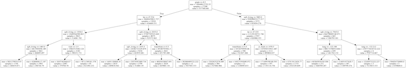
Note that the feature importances are interesting in that the top 5 include grade, sqft_living, lat, long and yr_built. All of these make sense but we have to note that lat and long were not strongly correlated with price. This is because they are not 'linearly' correlated with price and shows why a non linear model is important in this case.
Next we could try a more complex model: A GradientBoostingRegressor. This model has better performance, 0.861, and also happens to have feature importance capabilities. The top 5 features are pretty similar to the smaller decision tree but there are some position changes and yr_built has been replaced by waterfront.
Permutation Importance
What if a model did not have feature importance capability? For example if you wanted to use a neural net or a hand crafted ensemble of various kinds of models. Or perhaps we want to measure feature importance on different datasets such as in practice (the test set) versus just the importances discovered during training.
For this we can use a permutation importance tool such as ELI5. The idea is that you look at each feature in turn and shuffle the values in each column. This should destroy the predictive power of the feature while maintaining the same feature value distribution. The features who's shuffled values affect the model performance the most are most important. This simple technique works with any kind of model as long as you can shuffle the features individually and intelligently (ie. look out for one hot encodings).
perm = PermutationImportance(model).fit(X_train, y_train)
explore_feature_importances(perm.feature_importances_, X_train.columns)
Doing this yields a slightly different feature importance score. Notice that lat (proximity to Seattle) is even more important now.
Partial Dependence Plot (PDP)
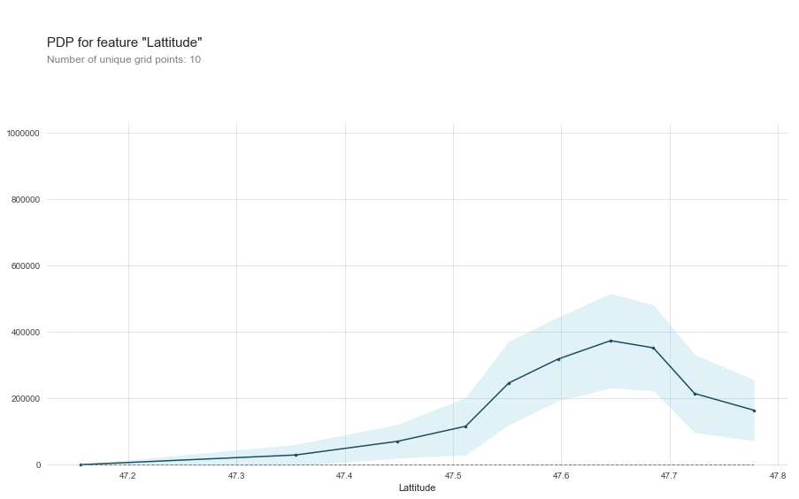
Along with randomly shuffling the values in a feature we can systematically change the value of one feature and keep the rest the same and note the affect on the prediction. For example if we do this with latitude we'd keep everything but lat the same and make predictions on all houses as if they were at one latitude and then at the next latitude and the next, etc. And then plot the result in a Partial Dependence Plot (PDP)
pdp_lat = pdp.pdp_isolate(model=model, dataset=X_val, model_features=X_train.columns, feature='lat')
fig, axes = pdp.pdp_plot(pdp_lat, 'Latitude')
The PDP shows us that the price of homes increases as it gets closer to 47.65 and then starts to drop off. Coincidentally Seattle's geo coordinates are 47.6062° N, 122.3321° W. The PDP even drops off sharply as we run out of data north of Seattle where King County ends. Typically PDP plots show a single line representing the mean change but PDPBox also shows a shaded area to represent variance. And it can even do multiple lines where each line represents an individual sample being moved through the space.
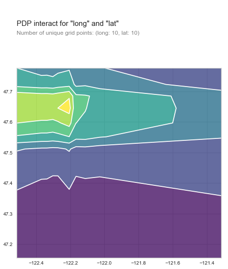
PDPBox even lets you plot two features at once. If we use lat and long together we can clearly see that houses would sell the most if they were in the north west corner of King county. Right where Seattle is. So if you want to get top dollar for your house move it there.
Local Interpretable Model-Agnostic Explanations (lime)
Next we look at approaches that claim that simple models can be used to 'locally' interpret more complex models. One recent approach that has gotten a lot of attention is Local Interpretable Model-Agnostic Explanations (lime). Given a trained model and a particular sample:
- generate random samples near the given sample
- weight generated samples based on proximity
- fit an explainable model to the generated data and predictions
- use the simpler trained model to interpret the predictions in the area of the sample
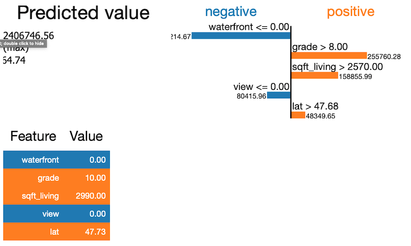
This lets you look at a particular sample and evaluate what led to the particular prediction by examining the local area around the sample. It also has the added benefit of estimation how much each feature contributed or detracted from the particular house.
In this example we examine one sample from the data and see that not being on the water front and not being viewed was a negative but the grade, sqft_living and lat was a positive.
Shapley Values
Finally, Shapley values, use a game theoretic approach to assigning attribution to features. The Shapley value is the average expected marginal contribution of one player after all possible combinations have been considered. Calculating Shapley values can be quite expensive but estimates have been developed, and implemented in SHAP, that speed the process with only a minimal loss in accuracy.
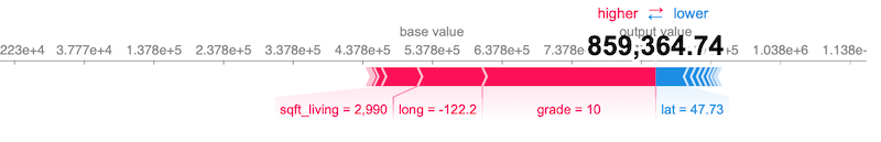
The chart can be a little tricky to read but it says that for this particular house the lat cost it ~$46k while the grade boost the price ~$250k and the long ~$93k.
Summary
- Explainability is why. Interpretability is how.
- Use Feature permutation (ELI5) instead of / along with feature importance.
- Partial Dependence Plot (PDPBox) show exactly how a feature affects the target.
- Shapley values (SHAP) are a game theoretic more precise way to measure effects.
- If you like R check out IML.
If you have any questions or comments get in touch.